Module 2: Deep Learning Basics

Optimization Basis

Training AI and machine learning models reduces to solving an optimization problem:

where is the loss function over model parameters . It typically takes the form

where is the loss contributed by a single data point .

The main challenge arises from the scale: modern deep learning involves billions of parameters and data points, making this a very expensive large scale optimization problem. The choice of optimizer directly affects the model’s final accuracy, training speed, and cost.

Gradient Descent

Gradient descent updates the parameters by moving in the direction opposite to the gradient of the loss:

where we start from an initialization and iteratively update by following the negative gradient direction.

The learning rate controls the step size. If it is too small, convergence is slow; if it is too large, the updates may overshoot or diverge.

Mini-batch Gradient Descent

For large datasets, the loss function in Eq. equ:lossform requires summing over many data points. Correspondingly, in gradient descent, computing the gradient involves evaluating the full sum:

Mini-batch gradient descent approximates this full-batch gradient by averaging over a smaller subset of data:

where is a subset of data indices, known as a mini-batch. The mini-batch may be drawn randomly at each iteration or selected sequentially by sweeping through the dataset. The batch size is .

An extreme case is when a single data point is used:

where is a random data point selected the -th iteration. This is known as stochastic gradient descent (SGD).

Using mini-batches introduces variance and noise in the gradient estimates. However, it significantly reduces computational cost per update and enables more frequent updates. In practice, it is often more effective to take many noisy steps than to compute a single precise but expensive update.

Momentum

In gradient descent, gradients can vary significantly across iterations; that is, the gradients and may differ substantially. This variation can result from noise, poor conditioning of the loss landscape, or large step sizes, and may cause the update direction to fluctuate sharply.

Momentum is a technique used to smooth the gradient across iterations. Instead of directly using the current gradient to update the parameters, momentum computes an exponentially weighted moving average of past gradients:

Unrolling the recurrence shows that is an exponentially weighted average of past gradients:

Typically, is set close to , such as . This means the current gradient contributes to the update, with the rest influenced by past gradients.

The main benefit of momentum is that it smooths out noise, encourages consistent update directions, and reduces oscillations. This often leads to faster and more stable convergence.

In fact, in the limit of a small step size, momentum corresponds to the physical dynamics of a ball moving in a potential field with friction. The momentum term captures the effect of inertia in this analogy.

Remark 2.1.

Recall that

Therefore, is a convex combination of as shown in Eq. equ:mtgt.

Nesterov Momentum

If is too close to one, can deviate significantly from . One approach is to add the gradient back and use a linear combination of the gradient and momentum for the update:

With a proper choice of , it is possible to smooth the momentum without de-emphasizing the contribution of the current gradient.

Adaptive Methods

Coordinate Imbalance

In neural network training, different parameters can have vastly different gradient scales; that is, the magnitudes of the elements in the gradient vector may differ significantly. As a result, some parameters may update too aggressively while others change too slowly, leading to instability. Note that this issue is distinct from the variation between and , which momentum seeks to smooth.

Signed Gradient

Signed methods address coordinate imbalance by applying the sign function to the gradient or momentum vector, equalizing the update magnitude across coordinates:

This is one of the most aggressive normalization approaches, as it forces all coordinates to have equal update magnitude. Consequently, the update depends only on the sign of the gradient or momentum, not its magnitude.

As a trade-off, smoother normalizations can be used, such as a soft variant of the sign function:

where

with . When , this reduces to the standard function.

Adam Optimizer

The Adam optimizer (short for adaptive moment estimation) combines momentum with adaptive scaling. A simplified version of Adam’s update rule is:

where and are exponential moving averages of the gradient and its elementwise square , respectively. The update uses the ratio , applied elementwise.

Note that when , we have and , and the update reduces to the softsign gradient. Hence, Adam can be viewed as Signed Gradient Descent, smoothed across iterations through the recurrence of the two moment estimates and .

Adam can also be interpreted as applying an adaptive scaling factor to softsign momentum:

The adaptive learning rate can be interpreted as a measure of gradient agreement across iterations. If the gradients are highly inconsistent (e.g., frequently changing sign) along a given coordinate, the magnitude of tends to be small due to cancellation, while remains relatively large. This results in a smaller , which slows down the update along that coordinate. Therefore, Adam automatically adjusts the step size based on gradient coherence, a key distinction from softsign momentum.

Bias Correction of Adam

Standard Adam implementation is slightly more complicate than what we wrote above:

Here, we introduce and as scaled by a factor of and .

To see why we may (or may not) need to introduce bias correction, consider the case where . Then the update of becomes:

Using the identity , the bias-corrected term is given by:

This shows that is a weighted average of . In particular, if all gradients are equal, then .

However, if we initialize (using an initial gradient estimate), then without correction becomes a convex combination of , and bias correction should not be applied.

Remark 2.2.

Hence, the need for this correction term is directly tied to initializing the momentum with , .

In practice, the bias correction becomes less important as increases, since as .

Regularization and Weight Decay

The Overfitting Problem

Large neural networks can memorize training data instead of learning generalizable patterns. This leads to excellent training performance but poor validation performance. Regularization is a standard technique to mitigate overfitting by discouraging overly complex models.

L2 Regularization and Weight Decay

L2 regularization is one of the most commonly used techniques. It is also known as ridge regression in the context of least squares. It adds a penalty term to the loss function:

Applying gradient descent to this objective yields:

The term is known as a weight decay. Rewriting this highlights the explicit weight decay effect:

It shrinks the parameters toward zero, encouraging smoother models that tend to generalize better.

AdamW

For adaptive optimizers like Adam, weight decay should be applied separately from the gradient update. This is implemented in the AdamW variant:

where and are the bias-corrected first and second moment estimates, as defined previously.

Note, however, that this is no longer equivalent to minimizing an L2-regularized objective.

This decoupled approach ensures consistent regularization across parameters and often leads to improved generalization performance.

Muon Optimizer

Adam normalizes updates coordinate by coordinate. Muon takes a different view: many important neural network parameters are matrices, such as the weight matrix of a hidden linear layer. Instead of only balancing individual coordinates, Muon tries to balance the update as a matrix.

The name Muon stands for MomentUm Orthogonalized by Newton-Schulz. A simplified version of the update is:

where is the gradient of a matrix parameter . The first line is momentum, as before. The second line approximately orthogonalizes the momentum matrix. Intuitively, this flattens the singular values of the update, so the update does not over-emphasize a few dominant matrix directions.

If is the singular value decomposition of the momentum matrix, exact orthogonalization would replace by . Computing this exactly with SVD is usually too expensive inside every optimizer step. Muon instead uses a few Newton-Schulz iterations, which are based on matrix multiplications and are much more suitable for GPUs.

The practical benefit is efficiency. In recent language model training experiments, Muon often reaches the same validation loss with fewer tokens or fewer training steps than AdamW. Its per-step update can be slightly more expensive than AdamW, but the improved sample efficiency can still reduce the overall training cost. This is why Muon has become interesting for modern LLM pretraining, where optimizer efficiency directly translates into saved GPU time.

The figure is a toy two-dimensional illustration. It treats the two plotted directions as a proxy for singular directions: momentum smooths the update, Adam rescales coordinates, and Muon-like orthogonalization flattens the update scale before applying the step.

In practice, Muon is mainly used for hidden two-dimensional weight matrices. Other parameters, such as embeddings, output heads, biases, gains, and scalar or vector parameters, are usually optimized with AdamW.

---

Neural Networks

A central goal in machine learning is function approximation: to learn an unknown function from observed data. In many real-world tasks, the true mapping between inputs and outputs is highly complex and cannot be described explicitly by hand-crafted formulas. Instead, we rely on data-driven approaches to approximate this mapping in a flexible manner. Neural networks provide a powerful and versatile class of function approximators that are particularly well-suited for high-dimensional and structured data.

We typically adopt a parametric approximation framework. This means that rather than searching over all possible functions , which would be infeasible, we restrict ourselves to a parameterized family of functions:

Here, the parameter vector encodes the adjustable components of the model, such as the weights and biases in a neural network. By varying , the hypothesis class can represent a wide range of candidate functions.

The learning problem is then formulated as an optimization task: find the parameter configuration that minimizes the expected loss between the predictions and the ground truth:

In this expression, the loss function quantifies the discrepancy between the model output and the true label . Typical choices include mean squared error for regression tasks or cross-entropy for classification tasks.

This formulation highlights the interplay between three key elements: the choice of function class (the architecture of the neural network), the loss function that reflects the task objective, and the optimization procedure used to adjust . Together, they form the foundation of modern neural network training.

From Linear to Nonlinear: Building Neural Networks

The simplest parametric model is the linear function:

This model is attractive for its simplicity and efficiency. Linear models can be trained efficiently, often with closed-form solutions in regression settings, and they provide clear interpretability: each coefficient reflects the contribution of the -th input dimension to the prediction.

However, despite these advantages, linear models have limited expressivity. They can only capture relationships that are linear in the input space, meaning they are fundamentally incapable of representing curved decision boundaries or complex nonlinear structures. This limitation makes them insufficient for most modern machine learning tasks, such as image recognition or natural language processing, where data exhibits intricate nonlinear dependencies.

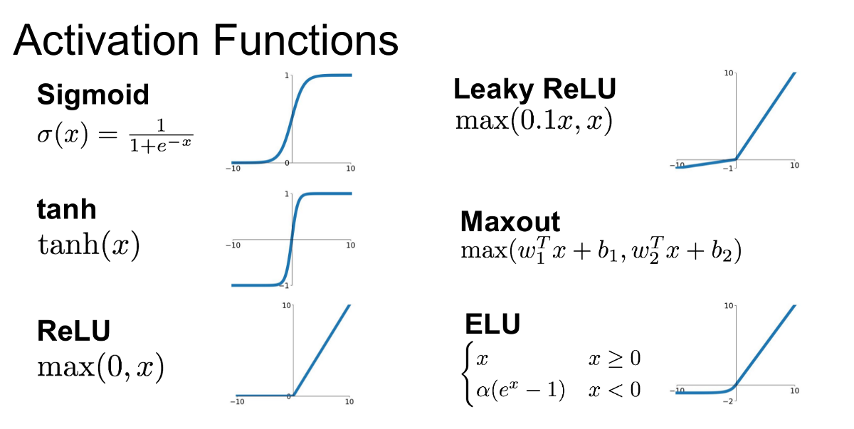
To overcome this limitation, we introduce neural networks, which generalize linear models by combining linear transformations with nonlinear activation functions. A single-layer neural network, also known as a shallow network, can be expressed as

where denotes a nonlinear activation function such as the rectified linear unit (ReLU), the sigmoid, or the hyperbolic tangent (). Each term in the summation corresponds to a neuron: a linear projection of the input followed by a nonlinear transformation, scaled by an output weight .

The introduction of nonlinearity is the key to increasing expressivity. Without , the composition of linear maps would remain linear, regardless of depth. With nonlinear activations, however, neural networks can approximate highly complex functions, enabling them to model intricate structures in data.

In this way, neural networks can be seen as building blocks: each layer transforms the input into a new representation, with nonlinearities ensuring that successive layers capture progressively richer patterns. This simple extension beyond linear models forms the foundation of deep learning.

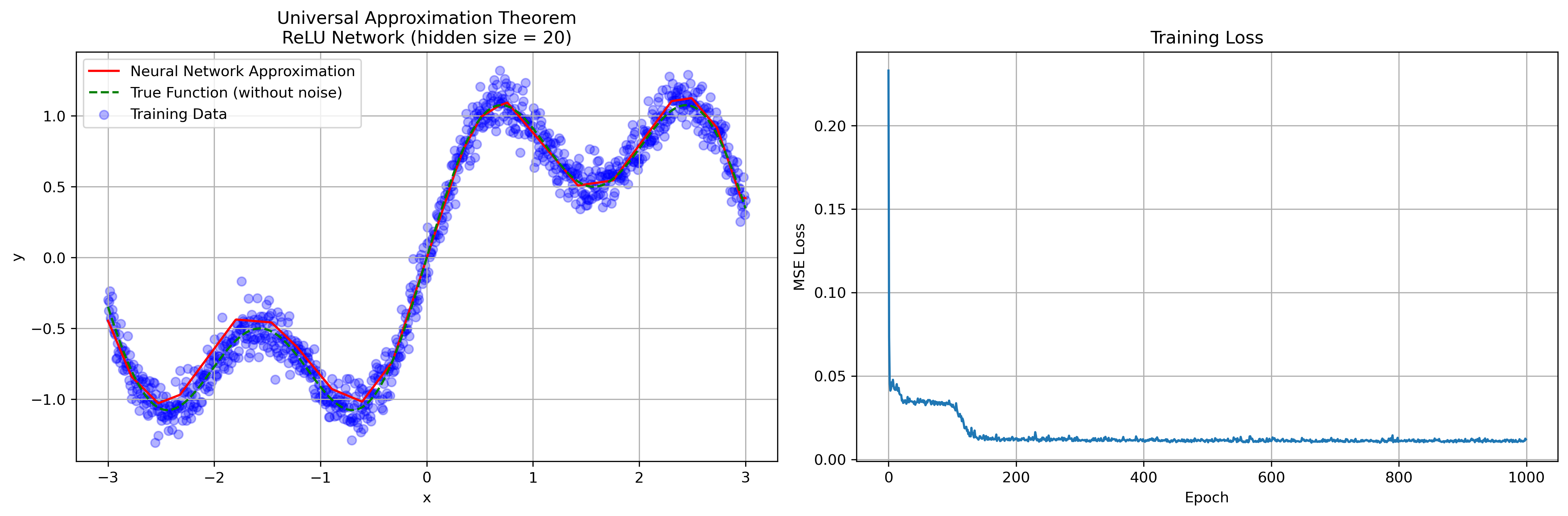
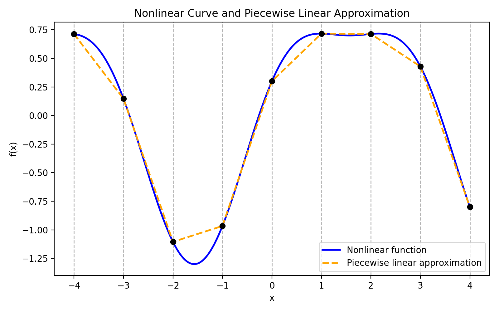
The figure shows a one-dimensional target function , the best linear fit, and a shallow neural-network fit . The lower strip shows the hidden units: each curve is one activated feature, and the output layer combines these features with learned weights to sculpt the final approximation. Here the output weights are fitted directly to highlight representational capacity, so the figure is not simulating gradient descent.

Universal Approximation Theorem

Theorem 2.1.

A neural network with a single hidden layer can approximate any bounded continuous function on a bounded domain to arbitrary accuracy, provided it has sufficiently many neurons:

More precisely, if is continuous and not a polynomial, then for any there exists and parameters such that

Assumptions and scope.

The statement is uniform approximation on compact sets: boundedness of and continuity of ensure and density is taken in the sup norm. The condition ” non-polynomial” excludes degenerate cases; popular choices such as ReLU, sigmoid, and satisfy it. Biases are essential---without them, the attainable set collapses on certain symmetric subclasses. The theorem guarantees existence of a good parameterization but is silent on how large must be, how to find by optimization, or how the required width scales with dimension.

Proof sketch (ReLU case).

1. Piecewise-linear reduction. Since is continuous on compact , for any there exists a piecewise-linear (PL) function such that (e.g., by triangulating and linearly interpolating nodal values).

2. ReLU realizes PL functions. In one dimension, a ReLU atom creates a kink at . Finite differences of shifted ReLUs synthesize hat/bump functions, e.g.,

which is triangular on and zero outside; summing such bumps reproduces any 1D PL function exactly. In higher dimensions, PL functions are piecewise affine on a polyhedral complex; each region can be carved out by maxima of affine forms and expressed as sums of ReLU of affine functions. Therefore there exists a one-hidden-layer ReLU network with , yielding by the triangle inequality.

Intuition.

Each neuron implements an affine projection followed by a nonlinearity, introducing a kink (ReLU) or a smooth bump (sigmoid/). By superposing many such localized shape primitives, the network sculpts increasingly fine features of until the uniform error falls below any prescribed tolerance.

Why not polynomial?

If were a polynomial, then any finite linear combination remains a polynomial in the input coordinates (after expansion). The hypothesis class would then coincide with a finite-degree polynomial family, which is not dense in under the sup norm unless degree tends to infinity. The non-polynomial condition prevents this collapse and ensures density.

What the theorem does not say.

It does not provide approximation rates in terms of smoothness of , nor does it claim that the required width is moderate--- can scale poorly with input dimension and target complexity. It also does not address statistical generalization or optimization; a representable may be difficult to learn in practice. Finally, for discontinuous targets one typically resorts to approximation on instead of uniform approximation.

Depth vs. width.

While the theorem uses a single hidden layer (width-driven expressivity), increased depth can represent certain function families with exponentially fewer neurons. Thus, depth trades width for hierarchical composition, often yielding superior parameter efficiency in practice, even though universality already holds at depth .

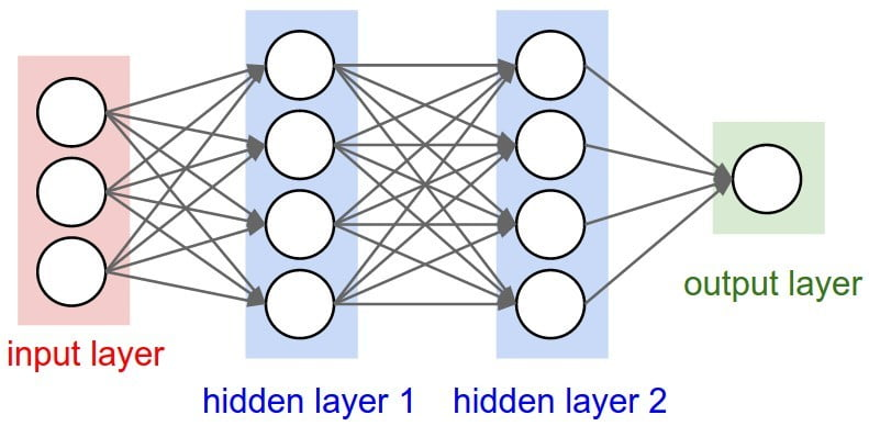
Deep Neural Networks: Composition of Functions

Instead of wide single-layer networks, we can build deep architectures by stacking multiple layers together:

Here, each layer is itself a nonlinear transformation, typically a linear projection followed by an activation function. By composing such transformations, deep networks successively refine the representation of the input: the early layers extract simple patterns, while later layers encode higher-level features.

The key distinction between shallow and deep models lies not in their theoretical ability to approximate functions (both can be universal approximators), but in the efficiency and structure of that approximation. Depth introduces a hierarchy that allows complex functions to be expressed more compactly.

Pros of Depth

• Composition matches the data. Real signals are built in layers: pixels become edges, edges become parts, parts become objects; tokens become phrases, phrases become meaning. Depth gives the model the same kind of compositional workspace.

• More expression per parameter. A shallow network can approximate many functions, but it may need enormous width. A deep network can reuse intermediate features, so small transformations can combine into a very rich function.

• Better inductive bias. Depth encourages progressively more abstract features. When the task has structure, this often helps the model generalize instead of memorizing every pattern separately.

Cons of Depth

• Harder optimization. Every extra layer is another transformation that gradients must cross. Without good initialization, normalization, and residual paths, signals can vanish, explode, or become noisy.

• Depth is not automatically useful. Adding layers only helps if they learn useful refinements. A poorly designed deeper model can train worse than a shallower one.

• More compute and fragility. Deeper models usually cost more memory, more latency, and more tuning. Architecture details start to matter a lot.

Colab Python Notebook

Residual Connections (ResNet)

The key idea of ResNet is to make each block learn a correction to a pass-through signal, rather than learning the whole transformation from scratch. If the desired mapping is , write it as

so the block computes

If the input and output dimensions do not match, the shortcut is projected instead:

Figure 2.1. Residual block: the main branch learns F(x), the shortcut carries x, and the block outputs x + F(x). Source: Wikimedia Commons / D2L, CC BY-SA 4.0.

This changes the optimization problem. If an extra block is not useful, it can make and behave like the identity. That is much easier than forcing a stack of nonlinear layers to learn the identity mapping exactly. This is why residual connections address the degradation problem: deeper plain networks can have worse training error, while residual networks give depth a safe fallback.

In classic ResNets, is a small convolutional subnetwork. ResNet-18 and ResNet-34 use a basic block: roughly convolution normalization/ReLU convolution, then add the shortcut. Deeper versions such as ResNet-50, ResNet-101, and ResNet-152 use a bottleneck block: convolution to reduce channels, convolution to process spatial structure, then convolution to restore channels. The shortcut is identity when shapes match, and a learned projection when resolution or channel count changes.

The practical lesson is that depth works best when each layer only needs to make a useful refinement. Residual blocks preserve an easy path for information and gradients, let layers start near identity, and make very deep networks trainable without asking every block to reinvent the representation.

Attention Mechanism

Modern architectures introduce the attention mechanism. Given a query vector and reference vectors , the attention output aggregates the values with data-dependent weights:

where the weights are obtained by a softmax over similarity scores

Here are linear maps producing query, key, and value representations. The softmax normalization makes the weights nonnegative and row-stochastic (sum to ), so the output is a convex combination of the values. Intuitively, tests which references are most relevant to the query via inner products with the keys , and determines the content to be aggregated. This decoupling between matching () and content () is the core advantage over fixed, position-only averaging.

From a matrix viewpoint, if we stack queries into and keys/values into , attention forms an weight matrix by row-wise softmax of , then multiplies by . The operation is differentiable end-to-end and adapts the receptive field based on content rather than fixed geometry.

In the figure, click a token to make it the query. The token row shows where attention flows, the heatmap shows the softmax weights formed from , and the value mixer shows how those weights average the vectors into one output. The numbers are hand-designed for intuition, not taken from a trained Transformer.

Self-Attention and Multi-Head Attention

Multi-Head Attention

Attention can be extended with multiple heads to allow the model to focus on complementary relational patterns:

where each head has its own and an output projection . Using multiple heads encourages the network to learn distinct similarity notions (e.g., syntactic vs. semantic relations in language) by projecting inputs into different subspaces before computing attention. The outer projections then mix these head-specific summaries into a single representation.

Self-Attention

In self-attention, every element serves simultaneously as a query and as a reference:

Each position aggregates information from all positions , enabling direct long-range interactions without stacking many local operations.

Properties.

• Permutation structure. As a set operation, self-attention is permutation equivariant to the order of inputs; it becomes order-aware once position information is injected (see below). Global pooling of self-attention outputs yields permutation invariance.

• Long-range dependencies. Every token can directly attend to any other token in one layer, providing a content-adaptive receptive field.

• Rich information exchange. Attention weights form data-driven routing of information across elements, allowing the model to emphasize salient interactions while suppressing irrelevant ones.

Homework

Homework 2: Optimization and Neural Networks