Problem 1
Problem 2.1 (Gradient Descent on Toy Quadratic Function).Consider applying gradient descent with constant step size on the following two-variable quadratic loss function:
The gradient descent update is
where
is the step size, and and are the gradients of with respect to and . Here are optimization variables, not data points. By varying
, the algorithm exhibits very different behaviors. For simplicity, assume throughout this problem; the case is similar in spirit. Answer the following questions with a mix of mathematical derivation and coding.
Let
be the parameters after iterations of gradient descent with constant step size and initialization . Since is quadratic, write down a closed-form formula for in terms of , , and . Derive this formula explicitly. There exists a critical step size
with the following properties:
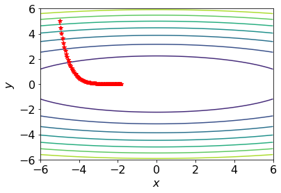
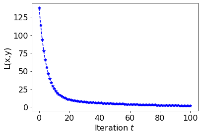
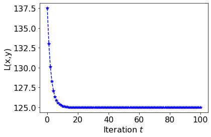
- If
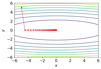
, the loss decreases monotonically to zero. - At
, the -coordinate converges to zero in one iteration. Derive
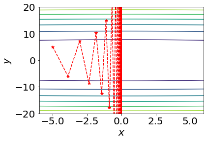
and show your reasoning. Also explain why the trajectories in the monotone cases exhibit an L-shape rather than moving straight to the origin. There exists another critical step size
beyond which gradient descent fails to converge. Derive and explain the cases below:
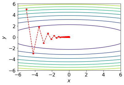
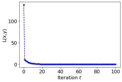
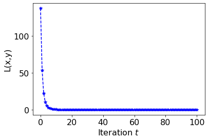
- If
, the trajectory converges with damped oscillations. - If
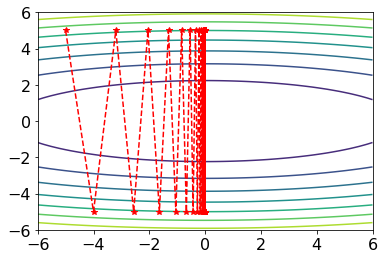
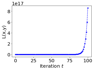
, the trajectory oscillates indefinitely with constant amplitude. - If
, the trajectory diverges with growing oscillations. Implement gradient descent for this example and reproduce contour plots similar to the phase reference above. Use
and . The plots do not need to be exactly the same, but they should qualitatively match the different phases. You may use this Colab contour plotting example. Write down the Adam optimizer update rule for this toy problem.
Implement Adam on the same quadratic function with
and . Vary Adam’s learning rate (denote it by to distinguish it from the gradient descent step size ) from very small to very large, and observe how the behavior changes. Comment on what you observe and how it differs from, or resembles, gradient descent. You may choose other Adam hyperparameters, such as and , freely. Optional. Assume we will terminate the algorithm at iteration
. Decide the best choice of step size so that the loss function is as small as possible at iteration . Precisely, choose an optimal step size such that is minimized. Note that:
- The optimal choice of
should depend on , , and the terminal iteration . - The optimal
never lies in the monotonic decreasing region and may exhibit damped or even undamped oscillation. By sacrificing monotonic decrease, we can take larger steps and make faster progress within iterations. In addition, derive the limit of
as . Optional. The studies above suggest that the efficiency of gradient descent decreases when
is very large. Consider the following approaches to speed up gradient descent:
Per-coordinate step size. Use different step sizes for different coordinates:
where
is the step size for and is the step size for . Describe a choice of and such that the algorithm reaches the minimizer within one iteration. Per-iteration step size. Vary the step size across iterations:
where the step size
depends on iteration . Show that, with a well-chosen step size scheme , gradient descent reaches the minimizer within at most two steps. Show your derivation.
Problem 2
Problem 2.2 (Optimizers on a Nonconvex 2D Landscape).Implement and compare several optimization algorithms on a simple two-dimensional nonconvex test function formed by a quadratic bowl plus two Gaussian wells:
Complete the provided Colab by adding implementations of the following optimizers in code: GD, Momentum, SignGD, SoftSignGD, RMSProp, and Adam.
- Implementation. Finish the optimizer implementations in the Colab.
- Trajectory visualization. For each optimizer, draw a contour map of
over and overlay the optimization trajectory for steps. Use at least three different initializations, for example , and budgets . Mark the start with and the end with . Briefly describe qualitative patterns you observe. - Hyperparameter exploration and comparison. For each optimizer, explore the effect of hyperparameters such as learning rate
, momentum or decay parameters, and the number of steps . Try several starting points and different budgets, such as and . Record: Then compare the optimizers: under a fixed step budget, which optimizer performs best on average across the specified initializations? For this comparison, use one chosen hyperparameter setting per optimizer, report how you selected it, and average the final objective over initializations. Name the winners and intuitively explain why they did well in this setting.
- the final objective
under different hyperparameter choices, - whether the run converged to the left or right well,
- your best settings for each optimizer and the corresponding final performance.
Problem 3
Problem 2.3 (Implementing Gradient Descent on MLP).Implement a simple multi-layer neural network, also called a multi-layer perceptron (MLP), with gradient descent. Starter code is provided in this Colab notebook. You are also welcome to use other frameworks if you prefer.
The provided code only works for two-layer networks. Extend the function
mlpso that it can handle an arbitrary number of layers.Using your extended code, try networks of different sizes, both in depth and width. Report what architectures you tested and describe how network size affected training loss and test performance.
In the starter code, the weights are initialized by sampling from
with scale parameter . Try different values of , for example , , and . Comment on what you observe. What happens if is too small or too large? What initialization strategy can help alleviate the gradient vanishing problem? Replace the
ReLUactivation withSigmoidand repeat the training. You will likely find it harder to train the network withSigmoid. Give an intuitive explanation of why this happens. Then try to improve the result by tuning hyperparameters such as initialization scale, learning rate, and number of iterations. Report your best results and any insights.The mean square error is not always the best loss function. In the presence of outliers, the Huber loss is more robust, since it behaves like squared loss for small errors but like absolute loss for large errors. See the Wikipedia page on Huber loss.
- Understand the logic of Huber loss and explain why it is less sensitive to outliers than the mean square loss. You may consult references.
- Modify the training data by introducing a few outliers, for example by setting the labels of the first five training samples to
. Keep the test data unchanged. Compare the performance of MSE and Huber loss on this dataset, and report your findings.