Module 6: Flow and Diffusion

Rectified Flow

Our goal is to learn a transport mapping that pushes a simple noise distribution to the data distribution . Classical approaches such as GANs, VAEs, and normalizing flows specify explicitly as a neural network, but each faces well-known training challenges: the minimax instability of GANs, the tension between reconstruction and regularization in VAEs, and the computational burden of exact likelihoods in flows.

We now discuss an alternative approach, in which is defined implicitly as the result of solving an iterative or continuous-time process whose local update is parameterized by a neural network. Such models are typically more flexible and can be easier to train because they only require learning local update directions, despite bringing higher computational cost in sampling.

Remark 6.1.

We distinguish two broad types of generative models:

• One-step models. The mapping is specified directly by a neural network, as in normalizing flows, GANs, and autoencoder-based models.
• Process models. The mapping is obtained by simulating an iterative or continuous-time process whose local updates are parameterized by a neural network, as in diffusion (SDE), flow (ODE), and autoregressive models.

In particular, in ODE (“flow”) generative models, we train a continuous-time process to gradually transform noise into a sample distributed as the data , assuming and have the same dimension. The dynamics are defined by the ODE

where the velocity field is a neural network with parameters . At each time , the field specifies the local update direction of the current state , and the interval serves as an artificial “time” along which noise is continuously transformed into data. Thus the model starts from a simple distribution at and evolves smoothly until it matches the data distribution at .

Integrating the ODE defines a mapping implicitly through . Because the flow transports points along continuous trajectories, the initial noise and the final output necessarily share the same dimension. Throughout, we assume the ODE admits a unique solution for every initial condition so that the forward trajectory is well defined.

Numerical Simulation of ODEs

Once the velocity field is trained, sampling from the model reduces to numerically solving the ODE to obtain . A simple discretization is the forward Euler method:

with step size . As grows, the discrete trajectory better approximates the continuous flow defined by the ODE.

Backward Integration and Inversion

Since the ODE admits a unique solution for each initial condition, the mapping is (approximately) invertible. This allows one to map a data point back to its noise counterpart by integrating the ODE in reverse. A backward Euler update takes the form

Starting from a sample at , we can step backward to . This reversibility is a key advantage of flow-based generative models and underlies their use in both sampling and likelihood estimation.

Maximum Likelihood Training of Neural ODEs

To understand how Neural ODEs can be trained by maximum likelihood, we consider the evolution of probability densities along the continuous flow induced by the ODE. Let denote the density of the random variable obtained by integrating

up to time . Thus represents the pushforward of the base density under the flow map defined by the velocity field .

A key property of continuous-time flows is that the log-likelihood admits an explicit expression in terms of the divergence (trace of the Jacobian) of the velocity field. If is the ODE trajectory that ends at , then

This relation shows how the likelihood of a data point evolves as it is transported backward along the flow from time to time . The formula is the continuous-time analogue of the change-of-variables formula for normalizing flows, where the determinant of the Jacobian is replaced by the time integral of the divergence.

Maximum Likelihood Estimation

Given the expression above, one can in principle train the Neural ODE by maximum likelihood. For data sampled from the empirical distribution , the objective takes the form

where is computed by tracing the flow backward to time and accumulating the divergence of the velocity field along the way. This approach is described in detail in .

Practical Challenges

Although conceptually elegant, maximum likelihood training of Neural ODEs is computationally demanding. Each evaluation of the log-likelihood requires solving an ODE trajectory, and backpropagation involves differentiating again through this ODE solution. As a result, both forward and backward passes are significantly more expensive than in discrete normalizing flows.

Another limitation is that the optimal velocity field is not unique: many different flows can transport the base distribution to the same target distribution with equal likelihood. This non-uniqueness complicates optimization and can lead to training instabilities in practice.

Rectified Flow: A Simpler and Better Approach

Although Neural ODEs can be trained using maximum likelihood, the approach is computationally heavy and difficult to optimize. It took several years of research to realize that there exists a much simpler and often better approach---one that is essentially simulation-free and avoids solving ODEs during training.

This insight first emerged from the study of diffusion generative models. Denoising diffusion probabilistic models (DDPMs) revealed that stochastic differential equation models could be trained by directly matching denoising behavior, and later developments such as denoising diffusion implicit models (DDIMs) demonstrated that these stochastic processes could be associated with deterministic ODEs. Similarly, score-based generative models were shown to correspond to a deterministic probability flow ODE, offering a new route to generative modeling without explicit simulation of stochastic dynamics.

These ideas were soon simplified and generalized into a family of formulations, including rectified flow, flow matching, and stochastic interpolants. All of these frameworks share the same principle: instead of learning an ODE by maximizing likelihood, one directly learns a velocity field that transports data and noise along simple, analytically chosen reference paths.

Rectified Flow

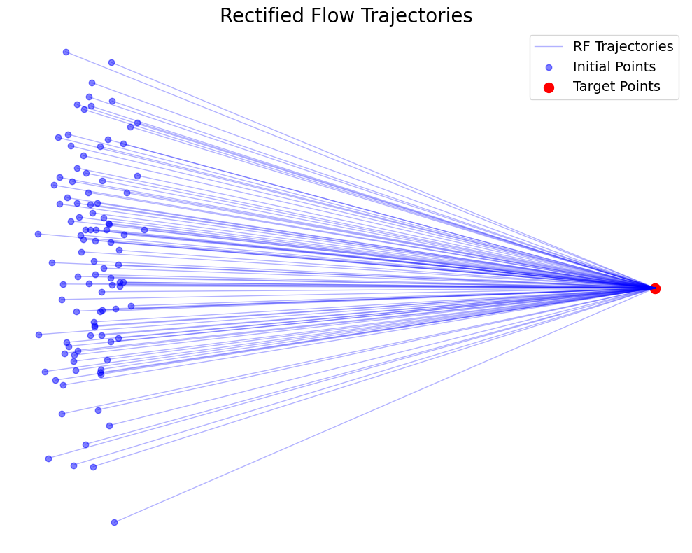
To build intuition, consider the simplest case of transporting a single data point . Starting from a random noise sample , we ask a basic but instructive question:

What is the most natural ODE that moves to ?

A natural choice is to use straight-line paths connecting noise and data. This geometric intuition leads to the so-called straight interpolation,

which traces the shortest path between the starting point and the target point .

To derive the corresponding ODE, we differentiate the interpolation:

Since the ODE must be expressed in terms of the current state , we substitute , which yields

This identifies the ideal velocity field for straight-line transport:

The scaling factor guarantees that all trajectories reach the target point exactly at time . Thus, rectified flow provides an analytically simple and geometrically intuitive velocity field, circumventing the complexities of likelihood training and numerical ODE simulation.

Rectified Flow: Straight-Path Dynamics

For a single data point , the rectified flow formulation identifies a simple and fully explicit ODE that transports a noise sample to the target . Using the straight-line interpolation

we can compute its time derivative and obtain the ideal dynamics

This ODE exactly reproduces the straight path for every , and it guarantees that the trajectory arrives at the destination at time .

An appealing property of straight-line dynamics is that their numerical discretization is extremely simple. A single forward Euler update,

recovers the exact endpoint of the continuous path. Thus, the trajectories are not only perfectly straight but also exactly realizable with a one-step discretization.

To learn such dynamics with a neural network, we introduce a parametric velocity field and choose a loss that encourages the model to match the ideal velocity along the straight interpolation between noise and data.

This leads to the objective

which, after substituting , can be written as

with . This simple regression objective captures the essence of rectified flow: the model only needs to fit the analytically known straight-path velocity, avoiding all simulation or likelihood computation.

Rectified Flow with Multiple Data Points

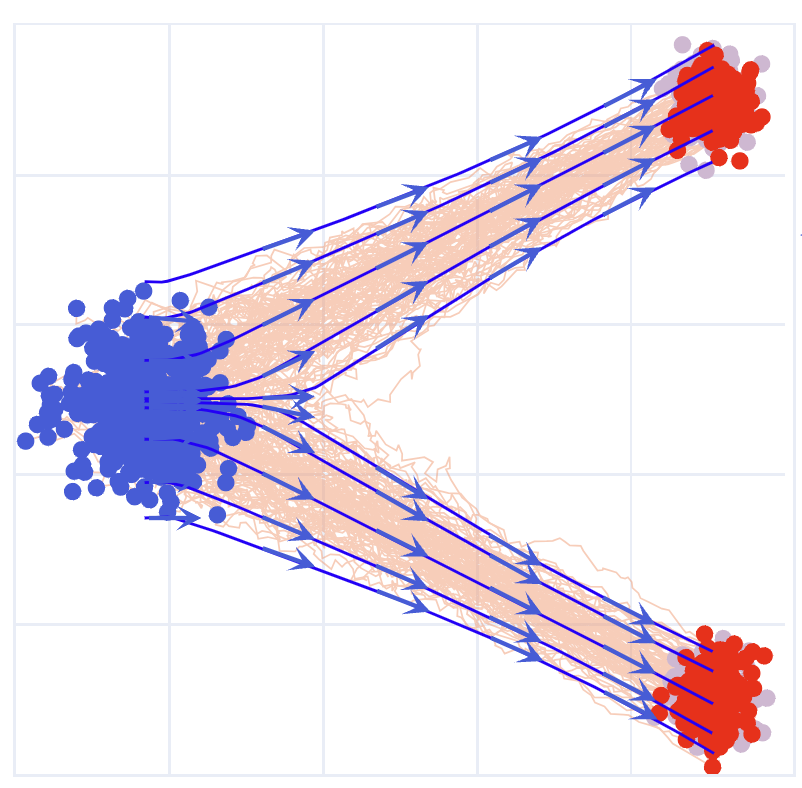
The single-point case suggests a clean formulation of straight-path dynamics, but real data consist of many points. To understand how rectified flow generalizes, consider several data—noise pairs simultaneously. Suppose we draw two independent pairs and . Each pair induces its own straight-line interpolation,

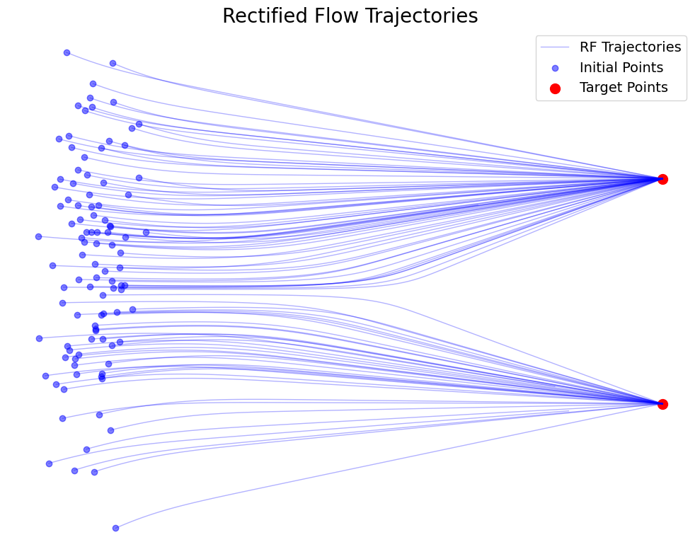A difficulty appears immediately: straight-line interpolations from different data—noise pairs may intersect. That is, for some time and some point ,

However, intersections of this form are impossible for the trajectories of an ODE. If a point lies on a trajectory of an ODE , then its instantaneous slope is uniquely determined by the velocity field . Thus, two different trajectories cannot pass through the same point with different directions, and naive linear interpolation does not define a valid ODE.

This raises the key question:

Can we convert linear interpolation into a valid ODE flow that respects the non-intersection property?

The resolution is surprisingly simple. Whenever trajectories intersect, we assign them a common direction by taking the conditional expectation of the ideal velocity at that point. Formally, we define the ideal velocity field as

where the expectation is over all data—noise pairs that interpolate to the same location at time . This averaging eliminates the inconsistency created by intersections and produces a well-defined ODE velocity.

To estimate this conditional expectation in practice, we again use a regression loss. Sampling independent pairs and , and forming , we minimize

This loss has a natural statistical interpretation. For any pair of random variables , the function is known to be the minimizer of over all measurable functions . Thus, the learned velocity field approximates exactly the conditional expectation defining the ideal rectified flow.

Rectified Flow Loss and Training Procedure

The rectified flow objective follows directly from the conditional expectation characterization derived earlier. Given independent draws and , and the straight-line interpolation

we define the rectified flow loss as

This regression loss trains the neural velocity field to approximate the ideal velocity , thus constructing a valid ODE flow that interpolates between noise and data.

In practice, the integral and expectations are optimized using stochastic gradient descent. Each iteration draws a minibatch of samples

and forms the interpolated points

The instantaneous training loss for each sample is then computed as

and the parameters are updated using its gradient. This procedure provides an unbiased stochastic estimate of the full objective .

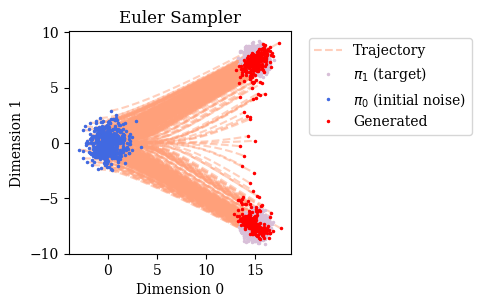
After training, the learned velocity field defines a generative model. Starting from a noise sample , one solves the ODE

transporting the initial noise toward the data distribution. The solution at time produces a generated sample , completing the rectified flow generative process.

Theoretical Properties of Rectified Flow

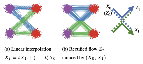
To analyze the behavior of rectified flow, consider independent noise—data pairs with and . The straight-line interpolation between them is given by

This linear path defines a simple time-indexed random process .

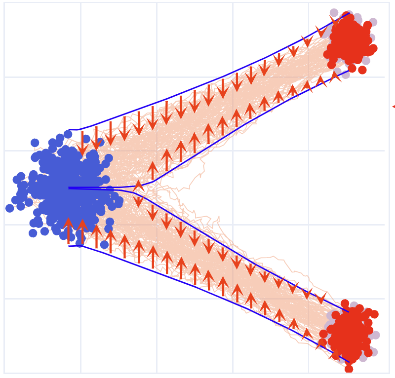
Rectified flow, on the other hand, induces a second process by solving the ODE

where the ideal velocity field is

This velocity field takes the average direction of all straight-line interpolations passing through any given point , ensuring that the rectified flow dynamics produce valid ODE trajectories.

Although the interpolation process and the ODE process are generally different random processes, a crucial property holds:

meaning that they share the same marginal distribution at every time. This agreement of marginals is a fundamental feature that enables rectified flow to match the data distribution while maintaining ODE-consistent dynamics.

Theorem 6.1.

Let denote the marginal density of either process or . Then satisfies the continuity equation

Here the divergence of a vector field is

If the continuity equation admits a unique solution for the given initial density , then both processes must share the same marginal distribution at all times. Thus, the rectified flow ODE and the linear interpolation induce the same family of marginals .

Proof of the Continuity Equation

To derive the continuity equation satisfied by the marginal densities , we begin by examining how the expectation of a smooth test function evolves over time. By definition,

This expresses the time derivative of the expectation in terms of the time derivative of the density.

We now compute the same derivative in a second way, using the dynamics of the process . Applying the chain rule gives

Using the tower property of conditional expectation,

Since is measurable with respect to , it can be factored outside the inner expectation:

By definition of the ideal velocity,

we obtain

Finally, we apply integration by parts:

assuming that vanishes outside a compact set so that boundary terms disappear. Equating this with the earlier expression for yields

Since this equality holds for all test functions , we conclude that the density satisfies the continuity equation

We have used the standard integration-by-parts identity

valid for smooth that vanishes outside a finite region.

---

Rectified Flow: ODE Generative Model

• Rectified Flow: Learning ODE generative models from interpolations
• Draw batches of samples:

• Construct interpolation between noise and data:

• Minimize the loss function:

• After training, generate new data by solving the ODE:

ODE vs. SDE Models

• ODE (Flow): Generate data by solving

• SDE (Diffusion): Generate data by solving

where is standard Brownian motion.

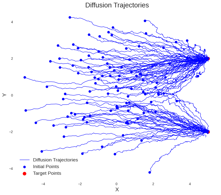
• SDE vs. ODE: How and Why?

Rectified Flow Recap

• Assume we have trained a rectified flow ODE model:

• Marginal preserving property: At each time , the distribution of matches the distribution of the interpolation

Thus, matches the data distribution .

• However, in practice, we cannot perfectly simulate the ODE due to model and numerical error.

Diffusion = ODE + Langevin

• If we know , we can correct errors using Langevin dynamics:

(Here, is an auxiliary time scale for Langevin correction at fixed .)

• Combine ODE and Langevin dynamics directly:

• Key: For Gaussian noise, the score function is directly related to :

Tweedie’s Formula

At time , let be the density of the interpolation

Then, Tweedie’s formula gives:

Proof

Proof. Given , we have , thus

Since , we have

Taking the gradient:

Recognizing the conditional expectation, we get:

◻

• On the other hand, the RF velocity is:

Thus, , and substituting this gives: