Recall that we aim to learn a mapping
We now turn to an alternative, autoencoder-based approach that relies on approximate invertibility. Instead of enforcing
The two networks are trained jointly to achieve approximate reconstruction,
allowing
We start with introducing the idea of autoencoders, which is general idea of using pairs of encoders and decoders for representation, and then discuss how to use autoencoders to build generative models such as variational encoders and adverairal antocoders.
Autoencoders: Non-Generative
flowchart LR
    X["input X"] --> Encoder["encoder E_phi"]
    Encoder --> Z["latent code Z"]
    Z --> Decoder["decoder D_theta"]
    Decoder --> Xhat["reconstruction X_hat"]
Structure of an autoencoder. The encoder (left) compresses input data
Example 5.1.In linear encoder—decoder models, we have
with
and , where are the dimensions of and , respectively. The autoencoder minimizes the expected squared reconstruction error: Let
, which has rank at most . Then the problem becomes This optimization has a closed form solution related to PCA/SVD.
Define
, and let be the eigendecomposition of the covariance matrix, where By the Eckart—Young—Mirsky theorem, the optimal solution above is given by the orthogonal projector onto the top-
eigenspace: A valid factorization achieving this
is obtained via: leading to the reconstruction
This is exactly the PCA reconstruction from the top
principal components. The minimum achievable loss equals the sum of the discarded eigenvalues (residual variance):
Equivalently, if the centered data matrix
has the singular value decomposition , the optimal linear autoencoder spans the same subspace as the top- left singular vectors .
Remark 5.1.Note that the solution of the autoencoder is not unique by definition. Given any encoder—decoder pair
, we can construct another pair with the same reconstruction mapping and hence the same loss. Specifically, for any invertible matrix , define where
denotes function composition. Then , so the reconstruction and the loss remain unchanged. This shows that the latent representation is only defined up to an arbitrary invertible linear transformation of the latent space.
An autoencoder (AE) learns to represent data through a pair of neural networks: an encoder
The training objective minimizes the reconstruction error:
Autoencoders are widely used for dimensionality reduction, denoising, and pretraining in deep learning. However, they are not inherently generative: the latent representation
Generative Autoencoders
Autoencoders can be made generative by introducing a regularization term that constrains the distribution of the latent variable
where
Different generative autoencoder variants are distinguished by the choice of the divergence
-
Adversarial Autoencoders (AAE) use a GAN-based adversarial loss to match
to . -
Variational Autoencoders (VAE) use the Kullback—Leibler (KL) divergence, with a stochastic encoder that enables a meaningful KL divergence computation.
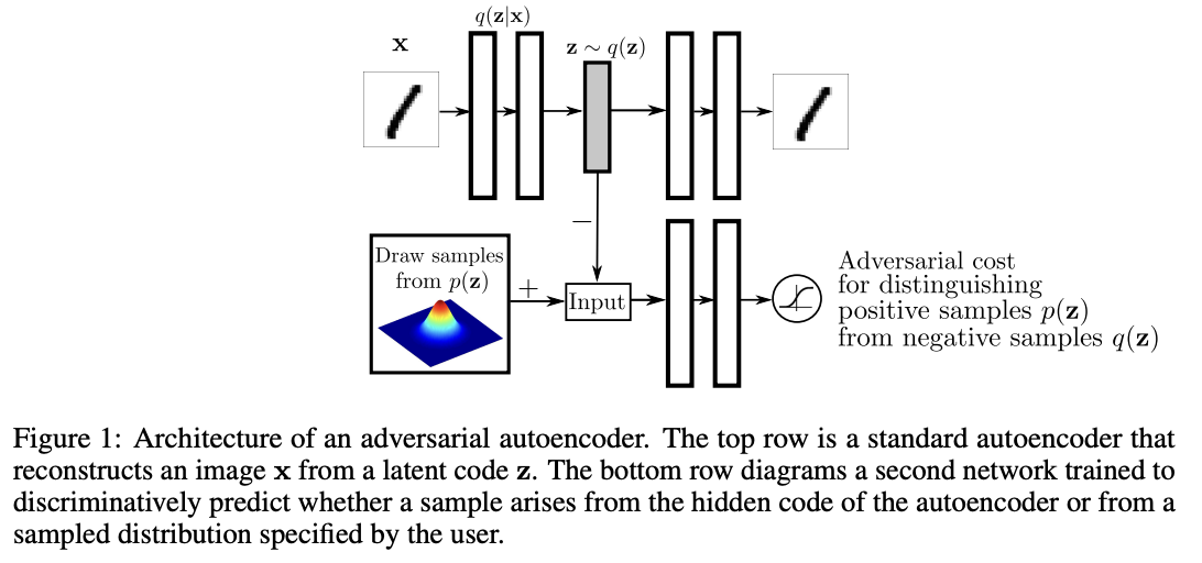
Adversarial Autoencoders (AAE)
The Adversarial Autoencoder (AAE) combines the reconstruction principle of autoencoders with the adversarial training mechanism of GANs to regularize the latent space. It enforces the encoded latent distribution
where
where
Full Objective.
The overall optimization becomes a min—max game:
This formulation integrates the reconstruction power of autoencoders with the distributional matching capability of GANs, yielding a model that can both encode data and generate new samples.
Variational Autoencoders (VAE)
The Variational Autoencoder (VAE) [Kingma & Welling, 2014] introduces a probabilistic formulation of the autoencoder by combining reconstruction with a KL divergence penalty:
Here,
Motivation.
The deterministic encoder
Stochastic Encoder.
Each input
where
To align with the prior
Remark 5.2.The divergence between two Gaussian distributions admits a closed-form expression:
Minimizing this yields
and .
Applying the formula above, the overall KL regularization between the approximate posterior and the prior is
Reconstruction Term.
Given this stochastic encoder, the reconstruction loss becomes
which measures how well the decoder
Overall Objective.
The VAE jointly minimizes the reconstruction error and the KL divergence:
where
The
The coefficient
See example code here.
VAE: Probabilistic View
We develop a probabilistic perspective of the Variational Autoencoder (VAE), viewing it as a latent variable model defined by joint densities over observed and hidden variables. The key challenge---marginalizing over latent variables---is addressed through variational inference, which converts intractable integrations into tractable optimization problems.
Latent Variable Models
Setup.
We observe data samples
where
Marginal Likelihood.
Since the latent variable
If both
However, in practice only
In words, we maximize the log-likelihood of what we observe, and integrate (marginalize) over what we do not.
However, for deep generative models, the integral in
VAE as a Latent Variable Model
Consider a latent variable model where the latent variable
or equivalently,
This stochastic formulation corresponds to a decoder network
Model Densities.
The corresponding densities are:
Hence, the joint distribution factorizes as
Learning.
If both
However, in practice we only observe
The integral over
Variational Inference: Integration
Quantities like marginal likelihood above requires to compute an integral of the form
which is typically intractable in high-dimensional latent-variable models.
Introducing an Auxiliary Distribution.
Let
This simple identity forms the basis of importance sampling and variational inference.
Applying Jensen’s Inequality.
Taking the logarithm of both sides and applying Jensen’s inequality gives
where the inequality holds because the logarithm is a concave function. The lower bound
Remark 5.3.For a random variable
and a concave function , and the inequality reverses for convex functions:
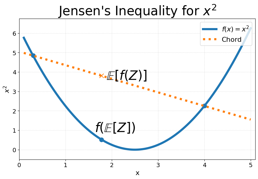
Illustration of Jensen’s inequality for convex (left) and concave (right) functions.
Gibbs (or Donsker—Varadhan) Variational Principle
The inequality in Eq. equ:logfineq becomes an equality when
To see this, note that for this optimal choice,
Combining Eq. equ:logfineq and Eq. equ:logfeq, we can express the logarithm of an integral as an optimization problem:
where
Further reformulation yields
where
This identity is known as the Gibbs variational principle, or Donsker—Varadhan representation, and is fundamental to variational inference. It shows that integration can be replaced by an optimization over distributions
Variational Inference for VAE
From the Gibbs variational principle, we have:
Applying this identity to the marginal likelihood of a latent variable model with
The distribution
The expression inside the maximization is known as the Evidence Lower Bound (ELBO):
Maximizing the ELBO jointly over
Expanded Form.
Since
where the first term encourages accurate reconstruction (expected log-likelihood) and the second term regularizes the latent posterior to stay close to the prior.
Joint Optimization.
In practice, both
This variational reformulation converts the intractable integral in