Module 4: Generative Adversarial Networks

Generative Adversarial Networks (GANs)

Given a dataset of i.i.d. samples from a target distribution on , our goal is to learn a parameterized generative model such that

produces samples that closely approximate . Here, is a simple reference distribution (e.g., standard Gaussian or uniform).

If the density function of the model output can be evaluated explicitly, we may estimate via maximum likelihood estimation. However, computing typically requires to be invertible and to have a tractable Jacobian determinant. This constraint motivates the use of invertible architectures, such as normalizing flows, specifically designed to ensure both invertibility and efficient density computation.

Generative Adversarial Networks (GANs).

An alternative approach is to give up the architectural constraint that the transformation must be invertible. In a GAN, can be any general neural network that maps latent samples to data samples . Since is typically non-invertible, the induced distribution of does not generally have a tractable or even well-defined density function. In fact, the probability mass of may concentrate on a low-dimensional manifold in the data space when is not invertible, making likelihood-based training infeasible.

To train such models, we must resort to likelihood-free approaches to estimate . A key idea is to train so that the generated samples match the statistics (or moments) of the real data. This leads to a class of moment-matching or adversarial training methods, which can be formulated as a minimax optimization problem, as we explain next.

Likelihood-Free Training via Moment Matching

Given a generative model , we can simulate a set of “fake” data points by pushing forward samples from the base noise distribution:

The goal is to find parameters such that the distribution of the simulated data matches that of the real data as closely as possible.

How can we tell if two datasets follow the same distribution? This is a classical two-sample testing problem in statistics. The idea is to compare various empirical statistics (or “moments”) of the two datasets.

For example, we can match the sample means:

However, matching only the mean is clearly insufficient. We can extend this idea by also matching higher-order moments, such as the variance. In the one-dimensional case, this corresponds to matching the second order moment:

This is, of course, still not sufficient unless the data distribution is Gaussian. To ensure that two general distributions match perfectly, we would ideally want to match all possible statistics, such as, all polynomial moments.

Figure 4.1. Examples of different distributions and their discriminator functions. Left: two distributions with the same mean but different variances. Right: two distributions with the same mean and variance, but different higher-order statistics.

This idea can be generalized by requiring that the generated distribution matches the data distribution on a rich class of test functions :

Here, the function class serves as a collection of test functions used to probe and compare the two distributions. If is sufficiently rich, then equality of expectations over all is enough to guarantee equality of the underlying distributions.

Definition 4.1.

A set of functions is called discriminative if it is rich enough such that matching the expectations over all implies equality of the distributions:

Example 4.1.

For distributions defined on , we have

where the choice of the function class determines which moments are being matched. Several important examples include:

Bounded Continuous Functions

Matching expectations for all bounded continuous functions guarantees equality of the two distributions.

Polynomials

If all polynomial moments agree, the two distributions coincide (under suitable regularity conditions).

Moment Generating Functions

Equality of moment generating functions implies that the distributions are identical.

Single-Neuron Neural Network

Here, is a nonlinear activation function, such as .

In practice, we may choose the test function class to be a family of neural networks. The example above shows that even a single neuron defines a valid test function for comparing distributions. More generally, multilayer neural networks provide a flexible and expressive class of test functions that can efficiently capture complex, high-dimensional relationships. They are also easy to implement and optimize using standard tools in modern machine learning.

Integral Probability Metrics (IPM)

Based on the moment matching idea introduced above, we can define a notion of discrepancy between the model distribution and the data distribution by maximizing the difference of test function expectations under a size constraint:

This family of divergences is known as the integral probability metric (IPM).

When is symmetric (i.e., ), we can remove the absolute value in the definition of the metric and write the IPM equivalently as

This simplification holds because, for any function , its negation also belongs to . Hence, the supremum of the absolute difference is equivalent to the supremum of the signed difference over all :

In other words, the symmetry of allows us to drop the absolute value without changing the value of the supremum.

Remark 4.1.

The supremum in the IPM definition can diverge if the test function is allowed to grow arbitrarily large or oscillate too rapidly. For instance, if with an unrestricted constant , then

which can be made arbitrarily large by increasing . Constraining (e.g., ) prevents this divergence.

Hence, must impose a constraint on the norm, magnitude, or smoothness of , such as equiring or ; see Table tab:ipm. Such constraints limit the “strength” of , ensuring that the IPM measures genuine distributional differences rather than the effect of scaling. Name Equivalent Formulation / Comment Total variation (TV) Maximum mean discrepancy (MMD) RKHS norm induced by a kernel Wasserstein-1 distance Kantorovich—Rubinstein dual form

: Examples of integral probability metrics (IPMs). Examples of integral probability metrics (IPMs). By choosing different function classes , the IPM reduces to various classical measures of distributional discrepancy.

Regularized IPM

In practice, it is common to add

Generative Adversarial Networks (GANs)

In practice, one often considers a parametric critic and introduces a regularized empirical approximation:

where we introduce a regularization term in which measures the magnitude or smoothness of the test function , and controls the strength of this regularization. The regularization term prevents the critic from growing without bound and helps ensure stability during optimization.

Training the generator then becomes a minimax problem:

This formulation captures the essence of adversarial training, in which two components (the generator and the critic) interact in a competitive optimization process:

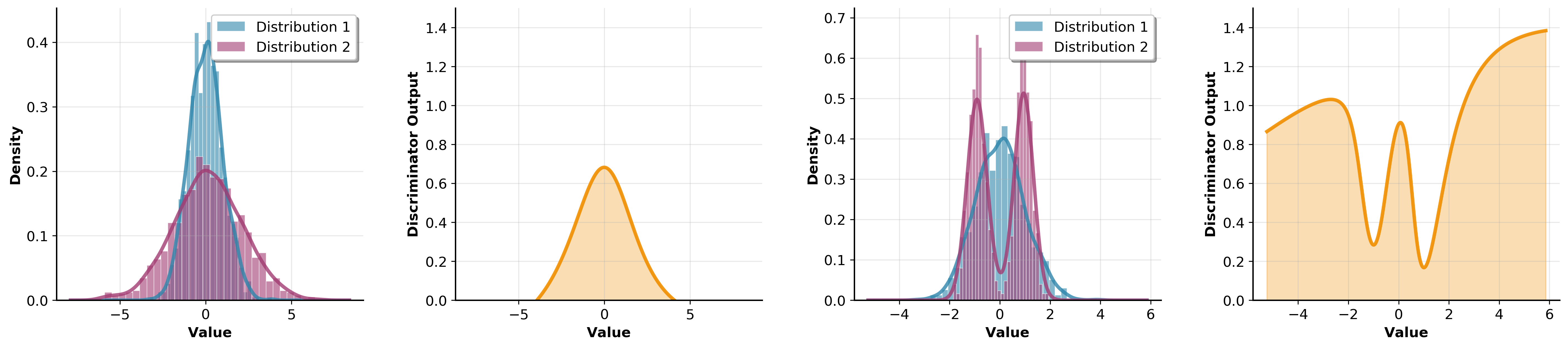
• Critic (or Discriminator) : Given the current generator , the critic seeks to find a test function that maximizes the discrepancy between the real and generated data distributions. Intuitively, the critic tries to distinguish real samples from fake ones by assigning higher scores to and lower scores to . The regularization term limits the critic’s expressiveness to prevent overfitting and ensure a well-defined optimization.

• Generator : The generator produces samples , where , and aims to minimize the discrepancy measured by the critic. In doing so, it adjusts its parameters so that the generated distribution becomes indistinguishable from the data distribution . When the minimax game reaches equilibrium, the generator has successfully learned to replicate the data distribution.

This adversarial structure underlies many modern generative models, including the Generative Adversarial Network (GAN), where the critic is typically implemented as a neural network, and the optimization alternates between updating and .

Classical GAN

The original GAN, proposed by Goodfellow et al. [@goodfellow2020generative], can be viewed as a special case of the IPM framework with an implicit convex regularizer defined by

where the convex function is given by

With this choice, the GAN loss becomes

where

Here, can be interpreted as the discriminator’s probability that the sample comes from the real data distribution. The discriminator is trained to distinguish real samples from generated samples , while the generator is trained to make them indistinguishable.

More generally, can be replaced by any other nonnegative convex function, leading to the broader -GAN family of models [@nowozin2016f].

Wasserstein GAN

The Wasserstein GAN [@arjovsky2017wasserstein] reformulates GAN training as minimizing the Wasserstein distance between the data and model distributions. This distance arises naturally from the integral probability metric (IPM) framework when the critic is constrained to be 1-Lipschitz continuous.

where the Lipschitz norm is defined as

Practical Implementation

In practice, the Lipschitz constraint is enforced approximately by constraining the parameters of the critic :

where controls the scale of the critic’s weights.

WGAN-GP

Weight clipping can restrict the critic’s capacity and lead to optimization issues. To address this, the improved WGAN by [@gulrajani2017improved] replaces the hard constraint with a gradient penalty (GP) that softly enforces the Lipschitz condition:

where

and

Here, is a real data sample, and is a generated sample drawn from the model distribution . The random interpolation coefficient ensures that lies uniformly along the straight line segment between a real and a generated point.

The gradient penalty encourages the critic to have gradients of unit norm along the straight line between real and generated samples.

Remark 4.2.

It is reasonable to use the following variance of gradient penalty:

which places penalty only when the gradient magnitude is larger than one, i.e., .

Solving Minimax with Alternating Gradient Descent

In general, GAN training can be formulated as solving a minimax optimization problem:

where

is the adversarial loss functional that couples the generator and the critic .

In practice, GANs are trained by alternating gradient descent, that is, by repeatedly updating the critic and the generator in turn using gradient-based optimization. A typical training iteration alternates between:

1. Critic update: Maximize with respect to (often for several steps) while holding fixed.

2. Generator update: Minimize with respect to using the most recent critic.

See the algorithm below for an illustration of this alternating update procedure.

Update critic parameters (with generator fixed):

Update generator parameters:

Remark 4.3.

Although the regularization term may depend indirectly on the generator through the generated data (for example, in WGAN-GP where depends on ), it is common practice to stop the gradient through when updating the generator. That is, we treat as a fixed quantity that does not backpropagate into the generator parameters .

A practical implementation of the improved WGAN algorithm is summarized below:

Given: dataset , prior , generator , critic , penalty weight , total iterations , and critic update frequency . Sample real data Sample noise , generate fake data Compute interpolation:

Update critic by minimizing

Sample noise , generate fake data Update generator by minimizing