Probability theory provides a mathematical framework for modeling uncertainty and randomness. We give a quick and informal overview of probability.
Probability and Random Variables
Random Variables and Distributions
A random variable (often abbreviated as RV) is a quantity whose value is determined by chance. Think of it as the outcome of a random device, like the roll of a die, or a process with inherent variability, like the mood of your cat.
While the outcome of a single trial is unpredictable, repeated observations of a random variable often exhibit stable statistical patterns. This idea is formalized through the notion of a distribution.
Suppose we repeat the random experiment times and observe outcomes . We denote the underlying random variable by an uppercase letter , and each observed outcome by lowercase , called a realization of .
The empirical measure is defined as
where is any subset of possible outcomes, and is the indicator function, which equals 1 if its argument is true and 0 otherwise. This expression gives the fraction of observations that fall within the set .
We typically assume that the observations are generated by repeated, independent trials of the same experiment, which is known as the i.i.d. assumption (independent and identically distributed). Under this assumption, it is reasonable to expect the empirical measure to stabilize as the number of trials increases. That is, for each measurable set , the frequency should converge to a limiting value:
This limiting function , which maps a subset to a probability scalar in , is a probability measure, or distribution of the random variable . It quantifies how likely it is for outcomes to fall within any set .
It is expected that a probability measure should satisfy the following basic properties:
for any sets on which is well defined (such sets are called measurable).
More generally, we can define the expected value of a function through its empirical average:
Here we write to be the integration of w.r.t. measure .
Discrete Random Variables
If is a finite or countable set, we can fully specify the distribution of by probability mass function (PMF) that gives the probability that takes the specific value :
The probability of any subset is obtained by summing:
As defined as limits of the empirical frequencies, we should obviously have and for all .
Continuous Random Variables
When is the Euclidean space , we can characterize the distribution with the probability density functions (PDFs), as the limit of probabilities over shrinking regions:
where is a ball of radius centered at , and is its volume. This limit may not exist, but if it does, the density function provides a full characterization of distribution of through integration:
We call that (and its distribution) absolutely continuous in this case. Similar to PMF, we should have and for all .
Examples
Example 1.1 (Uniform Distribution).
The uniform distribution on is a continuous distribution on with density:
It is denoted as .
Example 1.2 (Continuous and Discrete Gaussian Distributions).
The Gaussian distribution, denoted as is a continuous distribution on with density:
where is the mean and is the standard deviation, and is a normalization constant ensuring :
If we restrict the density on the set of integers , we get the discrete Gaussian distribution whose probability mass function is:
where the normalization constant is different from the continuous case. It does not have a closed formula like the continuous case.
Example 1.3 (Bernoulli and Categorical Distributions).
The Bernoulli distribution, denoted as , is a discrete distribution on with probability mass function:
The Categorical distribution is a discrete distribution on with probability mass function:
It is denoted as .
Example 1.4 (Hybrid Distributions).
Consider the following random variable:
It is a mixture of continuous and discrete random variables.
Building Complex Distributions
In practice, we often need to construct complex distributions from simpler distributions. This is fundamental to many areas of machine learning, including generative models, variational inference, and Monte Carlo methods. There are two different construction approaches.
Variable Transformation (Change of Variables)
Given a reference random variable , we can construct new random variables through deterministic transformations:
where is a measurable mapping. The resulting random variable follows a transformed distribution.
Theorem 1.1 (Change of Variables Formula).
If is continuously differentiable and invertible, and has density , then has density:
where is the Jacobian matrix of the inverse transformation.
The factor accounts for how the transformation changes the volume element.
Proof
For any measurable function , we have
On the other hand, we have
Matching this with Eq. , we get
◻
Intuition
Think of the formula as conservation of probability mass. A tiny interval around has mass approximately . After the map , that same mass occupies an interval of width . If the map stretches space, the mass is spread over more room and the density drops; if it compresses space, the density rises.
Remark 1.1.
Let , we have , where the first inverse is function inverse, and second is matrix inverse, and hence .
Example 1.5 (Log-Normal Distribution).
Let be standard normal, and define . By Theorem 1.1,
This gives the log-normal distribution, useful for modeling positive-valued data like incomes or stock prices.
Example 1.6 (Box-Muller Transform).
To generate samples from , we can use the Box-Muller transform. Let be independent, then:
are independent random variables.
Intuition
In polar coordinates, gives a uniform angle, so the cloud is rotationally symmetric; the radius has CDF , matching the radial distribution of a two-dimensional standard Gaussian; converting back to Cartesian coordinates gives the two normal coordinates.
Density Reweighting
Instead of transforming random variables directly, we may construct new distributions by modifying probability measures or density functions. A fundamental mechanism is density reweighting:
Here is called an importance weight function, and is the normalization constant ensuring that integrates to .
Example 1.7 (Gaussian Distribution with Different Means).
Let denote the density of the standard normal distribution . The density of can be written as a reweighting of :
The exponential weight shifts the mean from to while preserving the covariance.
Example 1.8 (Truncated Normal Distribution).
Let and define the weight
The resulting truncated normal distribution has density
where and denote the standard normal PDF and CDF, respectively. This construction restricts the support to and renormalizes the density.
Remark 1.2 (Importance of Normalization).
When modifying densities, proper normalization is essential. The constant guarantees that the reweighted function defines a valid probability density. Without normalization, would generally not integrate to .
Given a sample , how can we obtain a sample from ? Several general-purpose strategies are available.
Rejection Sampling
Assume that we can find a proposal density and a constant such that
An exact sample from can be obtained as follows:
draw ,
accept with probability
Upon acceptance, is distributed exactly according to . The main challenge is to find a tight bound . For example, if , then one requires . Tighter bounds lead to higher acceptance rates.
Self-Normalized Selection (Importance Resampling)
Rejection sampling yields exact samples but may be inefficient when is large. An alternative is an approximate method based on finite samples.
Draw i.i.d. from , and then select one of them using self-normalized importance weights:
This procedure produces an approximate sample from when is large.
Remark 1.3.
More precisely, the density of can be written as
where
By the law of large numbers, which implies Hence for large .
Markov Chain Monte Carlo (MCMC)
One can also avoid normalization altogether by constructing a Markov chain whose stationary distribution is . This leads to approximate sampling methods based on Markov chains, such as Metropolis—Hastings, slice sampling, or Langevin dynamics. MCMC methods trade exactness for flexibility and are widely applicable when direct sampling is difficult.
Mixture Distributions
Another fundamental mechanism for constructing new distributions is through mixtures. A mixture distribution combines several component densities into a single model:
where each is a valid probability density.
A sample of the mixture model can be obtained by first drawing an index to determine which component to select, and then drawing from .
Example 1.9 (Mixture Distributions).
Let and be mixing weights. The resulting Gaussian mixture model represents a multi-modal distribution whose mass is distributed among the Gaussian components. Sampling proceeds by first selecting a component index and then drawing
Other Distribution Transforms
Example 1.10 (Power Transformations of CDFs).
Let be a density function, and be its cumulative distribution function (CDF). For , we can define a new distribution:
This transformation creates a new density function that concentrates more mass in regions where is large when , and spreads it out when . The factor ensures proper normalization.
In terms of random variables, assume and define
so that . To generate a sample from , it suffices to draw
Indeed, since , the resulting random variable has CDF and density .
Learning Distributions from Data
In statistics and machine learning, we are given samples drawn from an unknown probability distribution and seek to recover the distribution that generated them. This distribution estimation task underlies density estimation, generative modeling, and many modern learning methods. It can be viewed as the inverse problem of probability theory: inferring the source distribution from its observed samples or induced properties.
Estimating a distribution from observations: samples are visible, the source distribution is hidden, and the learned model is an approximation.
Parametric Families
Consider a dataset of independent samples drawn from an unknown distribution:
where is the unknown true distribution governing the data generation process. Our goal is to estimate using a learning algorithm that takes the dataset as input:
To make this problem tractable, we typically assume that belongs to a known parametric family:
where represents the parameters of the model and is the parameter space. The problem then reduces to finding the optimal parameter that best explains the observed data.
Example 1.11.
For the data shown in the figure, it is reasonable to assume that follows a Gaussian distribution . In this case, the parameter vector is . A natural estimation approach is to use the empirical mean and variance:
These estimators have well-understood statistical properties and provide a solid foundation for understanding the underlying data distribution.
Example 1.12.
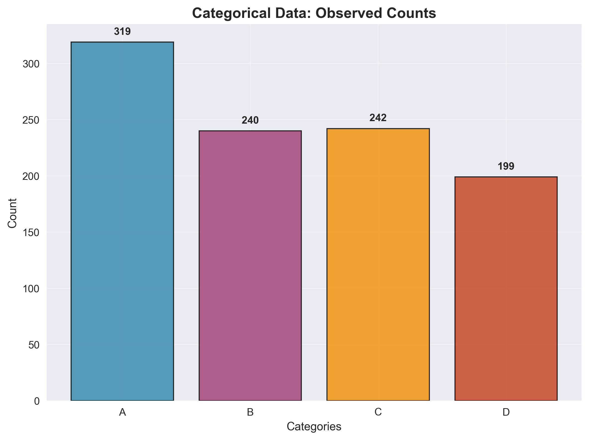
Consider a dataset of categorical variables, such as words in a text corpus or items in a shopping basket. Let be the set of possible categories. The data consists of counts for each category :
A natural model for this type of data is the categorical distribution with parameters where and . The maximum likelihood estimate is simply the empirical frequencies:
This intuitive result demonstrates how the data naturally suggests the appropriate parameter estimates.
Remark 1.4 (Inference vs. Learning: Key Distinctions).
The fundamental problems in probability theory, statistics, and machine learning can be viewed as converting between data and distributions.
Probabilistic Inference: Given a probability distribution, we infer its properties. Examples include calculating the mean, variance, or probabilities like from a known density function.
Sampling: Given a distribution , we draw i.i.d. samples from it. These samples allow us to estimate various statistics of the distribution, such as means, variances, and probabilities. Monte Carlo sampling can thus be viewed as a computational approach to probabilistic inference.
Learning (Statistical Inference): Given observed data , we estimate the underlying distribution. This can be viewed as the inverse problem of sampling. It is inference from statistics.
Density Models vs. Generative Models
There are two fundamentally different ways to represent a random phenomenon or distribution. The choice between these approaches has profound implications for both the mathematical formulation and the computational methods used in practice.
Density Models
Density models specify the probability function or probability density function explicitly. In this framework, we directly model the likelihood of observing each possible outcome:
where represents the probability function for discrete data and the density function for continuous data. This approach provides direct access to the probability values, making it straightforward to compute likelihoods and perform maximum likelihood estimation.
Example 1.13.
The Gaussian distribution is specified by its density function:
This explicit form allows us to directly evaluate the probability density at any point and compute the likelihood of observed data.
Generative Process Models
Generative models take a different approach by describing the procedure through which random variables are generated from a known random source. Instead of directly specifying , we define a generative process:
where is a simple base distribution (typically a standard normal or uniform distribution), and is a deterministic mapping, often implemented as a neural network. This approach focuses on the data generation mechanism rather than the resulting probability distribution.
Example 1.14.
We can represent Gaussian distributions in a generative way as the distribution of a random variable :
where samples are obtained by applying appropriate linear transformations to the standard Gaussian random variable . This generative perspective makes it easy to sample from the distribution and provides insight into the underlying data generation process.
Remark 1.5 (Inverse CDF Transform Sampling).
One-dimensional distributions provide another case where both density and generative representations are possible.
For a 1D distribution , we can represent it using its cumulative distribution function (CDF):
When is differentiable, we obtain the density function as .
When is invertible, we can generate samples from using the inverse CDF transform:
where is the inverse function of .
Intuitively, sample a vertical probability level , move horizontally until it hits the CDF curve, and then drop to the -axis. The shaded density area to the left of the returned is exactly .
This elegant relationship between density and sampling breaks down in higher dimensions.
The Trade-off Between Representations
Gaussian distributions and many other elementary distributions are special in that they admit both density and generative representations nicely. This means it is easy to both calculate the density and draw samples from the distribution.
However, Gaussian distributions are not capable of modeling complex data. For more complicated distributions, especially those defined using nonlinear functions such as neural networks, it is not easy to meet both conditions, and we need to make a hard choice on which representation to use.
Energy-based Density Models
One direction is to model more complex density functions using energy-based models. These models specify distributions whose densities are defined through a log-density function:
where is a neural network with parameters , and is the normalization constant that ensures is a valid density function satisfying .
By making a complex neural network, energy-based models can flexibly represent highly complex data distributions. However, these models suffer from critical computational challenges: the normalization constant is often intractable to compute, and even when learned, it remains difficult to sample from the resulting distribution . In other words, there is no straightforward generative process for sampling.
Neural Generative Models
Instead of using neural networks to model the density functions, we use neural networks to model the generative process:
where we choose as a neural network with as parameters.
This approach makes it easy to draw samples, but makes it hard to calculate the density. If the mapping is invertible, then we can also calculate the density using the change of variable formula:
However, this is not practical in high-dimensional cases, as it involves: (1) calculating the inverse of , (2) calculating the Jacobian matrix , and (3) calculating the determinant of the Jacobian matrix.
In general, if is not invertible, we need to estimate the density by calculating a complicated integration:
where is the density function of .
Parameter Estimation by Discrepancy Minimization
Regardless of which representation we use, the typical way to estimate the parameters is to minimize a discrepancy measure between the true distribution and our model :
where is a certain function that measures the difference between the true distribution and our model , such that if and only if .
In practice, we replace the unknown true distribution with the empirical distribution constructed from our data:
This empirical distribution places equal mass on each observed data point, providing a practical approximation to the true underlying distribution.
The key reduces to proper choice of the discrepancy measure that matches the (density or generative) representation of the model, in a way that renders tractable estimation even for complex models and high-dimensional data. Several discrepancy measures are commonly used in practice. The Kullback—Leibler (KL) divergence is perhaps the most fundamental, measuring the relative entropy between distributions. Other important measures include -divergences, integral probability metrics (IPM), Wasserstein distances, Fisher divergence, and kernel Stein discrepancy. Each measure has its own theoretical properties and computational characteristics, making the choice of discrepancy measure an important design decision in practice.
KL Divergence
Definition and Non-negativity
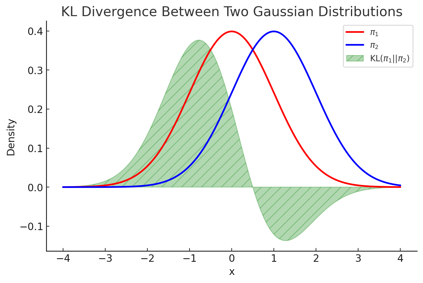
The Kullback—Leibler divergence between two distributions and is defined as:
Although not obvious at first glance, KL divergence yields a valid notion of discrepancy between two distributions: it is always non-negative,
with equality if and only if almost everywhere.
Remark 1.6.
Let’s walk through a quick proof that using Jensen’s inequality:
The key insight is applying Jensen’s inequality to the concave logarithm function. Recall that for any concave function :
The proof is completed by observing that , which follows from the fact that is a probability density integrating to 1.
This definition of KL divergence may seem mysterious at first glance. The non-negativity is not immediately obvious since we’re taking an expectation of log density ratios which can be negative for some values of . Yet remarkably, Jensen’s inequality guarantees that this expectation is always non-negative, regardless of the specific distributions and .
Example 1.15 (Numerical Example).
Consider two discrete distributions over three outcomes:
Let’s calculate the log ratio terms for each outcome:
The KL divergence is the expectation under of these log ratios:
Even though some log ratios are negative, their weighted average under must be non-negative, as guaranteed by Jensen’s inequality.
Interpreting KL Divergence
Let us develop another way to understand the non-negativity of KL divergence. We can consider the following obvious notion of discrepancy between two distributions and :
where is any non-negative function, which attains its minimum at . This obviously defines a valid notion of discrepancy with if and only if almost everywhere.
Example 1.16 (Chi-Squared Divergence).
A simple example of is , then
This yields the divergence.
Example 1.17 (Total Variation Distance).
Consider , we have
This yields the total variation distance.
To recover the KL divergence, we can choose
So we have
which recovers the KL divergence.
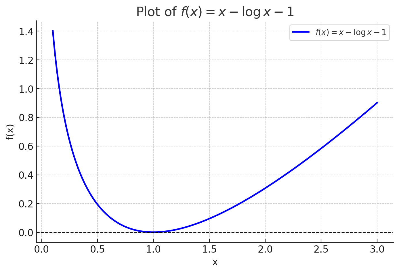
To verify that is a valid loss function, we examine its properties:
We have , , and for all . Therefore, is a non-negative convex function that attains its minimum at . See the figure for a visualization of the KL divergence.
Remark 1.7 (KL Divergence: Complete vs. Practical Forms).
The “complete” definition of KL divergence can be written as:
The term is theoretically zero (since ), and is “hidden” in typical definitions. In practice, we may or may not want to include it depending on the application context.
Remark 1.8 (f-Divergence: A General Framework).
Let be a convex function satisfying . Then, we can define a general family of -divergences:
This includes KL divergence as the special case when .
Similar to KL divergence, with equality if and only if almost everywhere. The non-negativity follows directly from Jensen’s inequality:
Alternative Representation: We can also express using the function
which is non-negative and convex. This leads to the equivalent form:
Key Insight: While must be convex for the original definition, the function provides an alternative representation where convexity is not strictly necessary for certain properties to hold.
Maximum Likelihood Estimation
KL Minimization and Log-Likelihood
A fundamental insight is that minimizing the KL divergence between the true distribution and our model is equivalent to maximizing the expected log-likelihood:
This equivalence can be seen by expanding the KL divergence:
The first term is the entropy of the true distribution , which is independent of . Therefore, minimizing the KL divergence with respect to is equivalent to maximizing the second term, which is the expected log-likelihood.
When we replace with the empirical distribution , this becomes the familiar maximum likelihood objective:
This equivalence provides a theoretical foundation for maximum likelihood estimation and explains why it is such a powerful and widely-used method.
Example 1.18 (Gaussian Maximum Likelihood).
For the Gaussian density , the log-likelihood function becomes:
When we maximize this function with respect to , we effectively minimize
whose minimum is attained at .
To find the maximum likelihood estimate of , we write and the log-likelihood function as:
Taking derivative with respect to gives
Setting it to zero, we get
Maximizing this function with respect to and leads to the familiar sample mean and sample variance estimators, demonstrating how the maximum likelihood principle naturally recovers intuitive parameter estimates.
Example 1.19 (Maximum Likelihood for Energy-based Models).
For energy-based models with density , the log-likelihood takes the form:
where
The first term encourages the model to assign high energy (low probability) to regions where data is sparse, while the second term acts as a regularization that prevents the model from collapsing to a single point.
Taking the derivative of with respect to gives
And
Combined, we have
which is the difference between the data and model based average (a.k.a. moment) of the gradient of . If , the gradient equals zero. Otherwise, the difference tells the update direction of the parameter as we perform gradient descent learning of :
However, the normalization constant is generally intractable to compute exactly, presenting a significant computational challenge that has motivated various approximation methods.